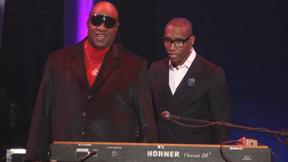
Most Popular


The EM Poll


browse back issues

All about Additive Synthesis

Feb 16, 2007 7:58 PM, By Scott R. Garrigus


         Subscribe in NewsGator Online   Subscribe in Bloglines
 

Putting sounds together one little piece at a time.

CURRENT NEWSSTAND ISSUE

Read the full Table of Contents for the issue on sale now! Click here

Subscribe for only $1.84 an issue!

Please tell us about yourself so we can better serve you. Click here to take our user survey.

MixBooks Logo
Life in the Fast Lane

This collection of St.CroixÕs columns was assembled during the two years following his death of cancer in May 2006. Included are many of his most-read columns, as well as personal notes, drawings and photographs.

Click for more books
EM Podcasts

Listen to these latest podcasts and more:
Bela Fleck on recording Jingle All the Way.Go

What's New: software and sound products. Go

eDeals Newsletter for Discounts on Gear

Get First Dibs on Hot Gear Discounts, Manufacturer Close-Outs and Job Opportunities when you sign up to receive eDeals E-newsletter, sent twice a month. Check out an issue get advertising info or subscribe

Most desktop musicians are familiar with the term "additive synthesis," but how many know exactly what it is and how it can be used to create sound? Like other methods of synthesis, such as subtractive, FM, or phase distortion, additive is a common technique that has great potential for synthesizing a wide range of sounds. In this article, I'll talk about the basic principles behind this technique and the different ways it has been implemented over the years.

To put it simply, additive synthesis is a sound generation technique that combines simple waveforms at various frequencies and amplitudes to create more complex, "composite" waveforms. Today's electronic instruments handle this task with ease, but additive synthesis actually dates back to the very beginnings of electrical theory.

Fig. 1: The simplest component of sound is the sine wave. This display shows a sine wave with a frequency of 440 Hz and an amplitude of 0 dB.

The Fourier Theorem

During the early nineteenth century, a French mathematician named Jean Baptiste Joseph Fourier theorized that any complex sound can be broken down into a series of simple sounds. The inverse of this is also true: any complex sound can be created by using the basic building blocks of sound. These building blocks are known as sine waves, and just as the atom is the smallest known unit of any element, the sine wave is the simplest known unit of sound. A sine wave is a pure, continuous tone with only one specific frequency and amplitude, such as 440 Hz at 0 dB (see Fig. 1). It is produced by any object that vibrates in a very simple pattern of back and forth motion, called sine motion. (It can also be produced electronically by nearly any synthesizer available today.)

Because the sine wave is so simple, however, it is also a very boring sound to listen to. You know that tone heard over your television at the end of the broadcast day? That's a sine wave. As Fourier's theorem states, the combination of multiple sine waves can create complex sounds, and that is the basis for additive synthesis.

The individual sine wave components that make up a complex sound are called partials, and each partial has its own unique frequency and amplitude. The range of these partials makes up the spectrum of the final sound. The first partial, called the fundamental frequency, is the most important because it determines the overall pitch and loudness of the sound. Each additional partial also influences the pitch and loudness but typically to a lesser degree. More importantly, these additional partials determine the timbre, or tone color, of the sound (see the sidebar, "The Timbre Story").

The Very First Synth

Unfortunately, during Fourier's day there were no practical means of testing out his theorem. It wasn't until the 1860s that Hermann von Helmholtz proved Fourier's theorem by making the first significant musical use of electricity. Helmholtz built an apparatus that consisted of a number of electrically driven tuning forks, each tuned to a specific partial. When played together, they produced a complex sound. This invention was the first "synthesizer," but it was by no means a musical instrument because it could only produce one specific sound at one specific pitch. (You can read more about the history of electric and electronic instruments in Joel Chadabe's excellent book Electric Sound, published by Prentice Hall, 1996.)

It wasn't long after the Helmholtz experiment, however, that American inventor Thaddeus Cahill created the world's first electrical musical instrument. Cahill's Telharmonium was also an additive synthesis-based instrument that combined simple sine waves to produce more complex sounds. The Telharmonium was a polyphonic instrument with a touch-sensitive keyboard that produced sine waves by using a series of rapidly spinning alternators. The alternators were driven by banks of electric motors that rotated at fixed speeds and controlled the frequency of the alternators and thus the pitch of the sound. The instrument predated the invention of the amplifier, however, and was a monstrosity that weighed over 200 tons and needed six railroad cars to transport. Because of this and other technological problems, the Telharmonium wasn't an enduring success.

B-4 the B-3

When Laurens Hammond took the rotating-disk system of the Telharmonium and combined it with more modern electrical technology, the first commercially successful electric musical instrument became available. The Hammond organ was invented in 1935 and first reached the public in 1939. It sported an electric motor that rotated a shaft containing 91 metal disks, each patterned with specific grooves, that were used to control note frequencies. Its additive synthesis-related features came in the form of switches called drawbars, each of which corresponded to a specific partial, and which together could be used to produce over 300,000 different sounds.

But the Hammond organ (along with its predecessors) still lacked two very important features for the creation of truly complex sounds. First, the organ produced sounds with nonvarying amplitudes, meaning you preset the volume of each partial and then every note had the same amplitude. The volume settings could be changed, but not while a note was sounding.

More serious, however, was the fact that the range of sounds the Hammond could produce was, in a sense, limited. Let's look at a little more theory to understand why.

Part and Partial

The partials that make up a sound's spectrum come in two forms: harmonic and inharmonic. Harmonic partials are defined mathematically as whole-number multiples of the fundamental frequency. For example, by doubling a fundamental frequency of 440 Hz, we get a harmonic partial with a frequency of 880 Hz, and tripling it produces another harmonic partial at 1,320 Hz. These frequencies are known as the second and third partials, and so on. Inharmonic partials, on the other hand, are those sine waves whose frequencies are not whole-number multiples of the fundamental. For example, partials at 500 Hz and 900 Hz would be inharmonic relative to a fundamental of 440 Hz. The Hammond organ was limited to harmonic partials, which is why it produced such pure and smooth tones.

To create truly complex sounds, any synthesizer should be able to produce both harmonic and inharmonic partials. And it should have the ability to combine several dozen to several hundred sine waves. Each of those waves requires its own oscillator, set to a unique frequency and amplitude. Because the loudness of most complex sounds varies over time, the amplitude of every sine wave must be dynamically controlled by an envelope generator. Each envelope generator requires at least an attack, decay, sustain, and release segment, so even with only 30 sine waves to manage, that's over 100 parameters that have to be controlled and created in real time in order to create a single note. This task was beyond the reach of any instrument in the 1930s and was something that could only be performed by the power of computing.

The Computer as Synth

During the 1950s and '60s, digital mainframe computers found in research institutions were first used to generate complex sounds by manipulating specific partials. Researcher Max Matthews at Bell Labs is credited with developing the first sound programming language. Matthews called his program Music I, and though the first version was a simple, 1-voice generation utility, it quickly evolved into an application that provided an unlimited number of voices. The program didn't work in real time, however. Sound parameters had to be fed into the computer, which then took a certain amount of time for processing, and the results had to be converted into an analog signal before being played.

Then, in the late 1960s, David Luce built a machine that would analyze a set number of partials for any complex sound and display their individual envelopes as plots on an oscilloscope screen in real time. These plots were photographed, and Luce would then manipulate the partials of the sound by redrawing the envelopes and having the machine scan his drawings (using an optical scanner). The machine would then play back the altered sound in real time. This was one of the first demonstrations of what is known as resynthesis.


Acceptable Use Policy
blog comments powered by Disqus

Get Copyright ClearanceWant to use this article? Click here for options!
© 2009 Penton Media, Inc.

Back to Top